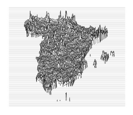
Las alturas corresponden a una cierta potencia de la población residente en la correspondiente rejilla. Los datos son del SEDAC (Socioeconomic Data and Applications Center, Universidad de Columbia) y se pueden bajar gratis si te registras y rellenas un cuestionario tontaina.
El código,
    library(ggplot2)
    options(expressions = 10000)

    dat <- read.table("dat/espp00ag.asc", skip = 6)
    dat <- as.matrix(dat)
    dat <- data.frame(y = as.numeric(row(dat)),
                      x = as.numeric(col(dat)),
                      pop = as.numeric(dat))

    peninsula <- dat[dat$x > 200,]
    peninsula <- peninsula[peninsula$y < 250,]

    res <- ggplot()

    for (i in 1:max(peninsula$y)){
      tmp <- peninsula[peninsula$y == i,]
      tmp$pop <- tmp$pop^0.3
      res <- res + geom_polygon(data = tmp, aes(x = x, y = pop - y), fill = "white", col = "black", size = 0.1)
      res <- res + geom_path(data = tmp, aes(x = x, y = pop - y), size = 0.2)
      res <- res + geom_hline(data = tmp, aes(yintercept = -y), col = "white")
    }

    res + theme(axis.line=element_blank(),
                axis.text.x=element_blank(),
                axis.text.y=element_blank(),
                axis.ticks=element_blank(),
                axis.title.x=element_blank(),
                axis.title.y=element_blank(),
                legend.position="none",
                panel.background=element_blank(),
                panel.border=element_blank(),
                panel.grid.major=element_blank(),
                panel.grid.minor=element_blank(),
                plot.background=element_blank())
Nota: se me olvidó escribir en el cuerpo lo que anunciaba el título, i.e., que esta entrada está inspirada (fusilada, de hecho) en lo esencial de otras previas.