Continúo en esta la primera de las entradas que hice sobre el artículo Don’t Be Loopy: Re-Sampling and Simulation the SAS® Way.
Trata sobre lo siguiente:
- Construir un conjunto de datos simples (dos vectores,
xey). - Hacer una regresión de
ysobrexy capturar los residuos. - Crear 1000 vectores
y'distintos añadiendo a $\hat{y}$ (la predicción dey) en el modelo anterior una reordenación de los residuos. - Crear los correspondientes 1000 modelos haciendo la regresión de cada $\hat{y}$ sobre
x. - Obtener el histograma del coeficiente de la regresión.
Es un caso de bootstrap en el que no se muestrean directamente los valores iniciales sino los residuos del modelo.
El código en SAS es el siguiente:
/* 0: data creation */
data temp1;
x=1; y=45; output;
do x = 2 to 29;
y = 3*x + 6*rannor(1234);
output;
end;
x=30; y=45; output;
run;
%let regressors = x;
%let indata = temp1;
/* 1: perform the regression and get the predicted and residual values */
proc reg data= &INDATA;
model y=®ressors;
output out=out1 p=yhat r=res;
run;
/* 2: split the data: only the residuals will require URS */
data fit(keep=yhat ®RESSORS; order) resid(keep=res);
set out1;
order+1;
run;
/* 3: this doesn't do any sampling - it copies the FIT data set repeatedly */
proc surveyselect data=fit out=outfit method=srs samprate=1 rep=1000;
run;
/* 4: this does the WR sampling of residuals for each replicate */
data outres2;
do replicate = 1 to 1000;
do order = 1 to numrecs;
p = ceil(numrecs * ranuni(394747373));
set resid nobs=numrecs point=p;
output;
end;
end;
stop;
run;
/* 5: then the randomized residuals are merged with the unrandomized records */
data prepped;
merge outfit outres2;
by replicate order;
new_y=yhat+res;
run;
/* 6: the bootstrap process runs on each replicate */
proc reg data=prepped outest=est1(drop=_:);
model new_y=®ressors;
by replicate;
run;
/* 7: and the sampling distribution is aggregated */
proc univariate data=est1;
var x;
output out=final pctlpts=2.5, 97.5 pctlpre=ci;
run;
proc print;
run;
que corre en mi máquina en 37.37 segundos.
Ofrezco dos alternativas sustancialmente más sucintas en R. La primera es una reinterpretación literal en R del código anterior,
    x <- 2:29
    y <- 3 * x + 6 * rnorm( length(x) )
    x <- c( 1, x, 30 )
    y <- c( 45, y, 45 )

    m0 <- lm( y ~ x )
    yhat <- m0$fitted.values
    res  <- m0$residuals

    resultados <- replicate( 1000, lm( yhat + sample( res ) ~ x )$coefficients[["x"]] )
    hist( resultados )
que corre en 2.46 segundos.
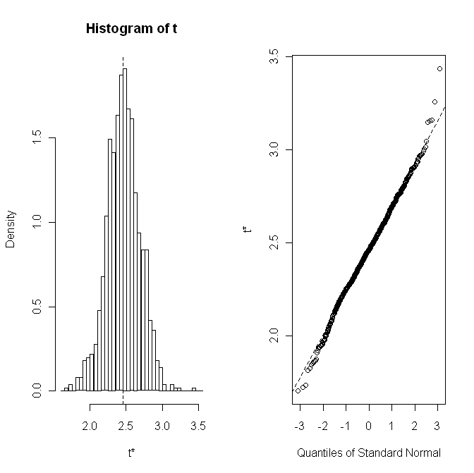
El segundo utiliza el paquete boot,
library( boot )

datos <- data.frame( y = yhat, x = x, res = res )

foo.boot <- function( datos, ind ){
    lm(y + res[ind] ~ x, data = datos)$coefficients[["x"]]
}

res <- boot( datos, foo.boot, R = 1000 )
plot( res )
que corre en 2.71 segundos.
El paquete boot es un candidato ideal para reimplementarlo utilizando paralelismo. Sin embargo, su mantenedor no parece estar por la labor. ¡Qué pena!